Tracking Time-Varying Beta & Latent States with Kalman Filters

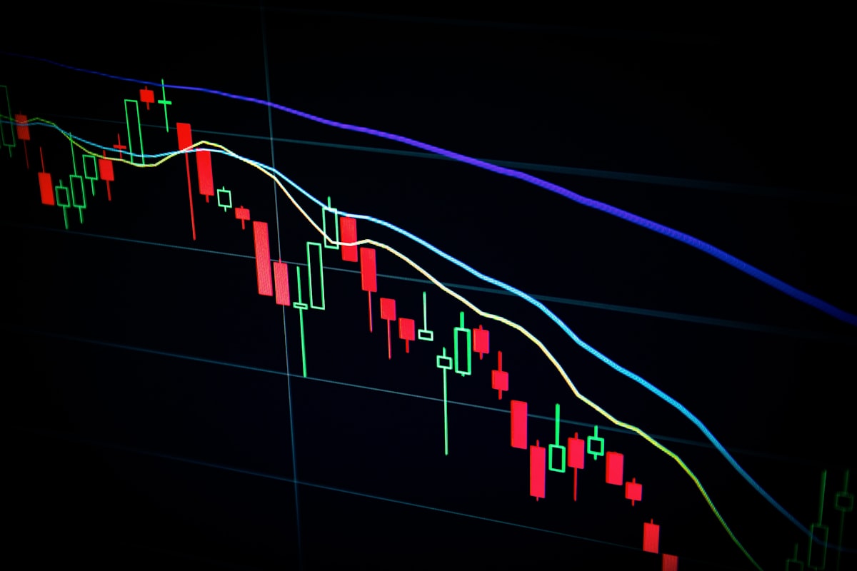
In financial econometrics and systematic strategy design, assuming that market parameters remain static over multi-year horizons is one of the quickest routes to strategy decay. Cross-asset correlations, hedge ratios, and asset betas are inherently non-stationary.

In this article, we examine how state-space representations combined with recursive Kalman filtering provide an elegant framework for tracking dynamic parameters in real time.

The State-Space Formulation

Consider estimating a dynamic hedge ratio or factor sensitivity $\beta_t$ between an asset return $y_t$ and a risk factor $x_t$. The measurement and state transition equations can be expressed as:

$$\text{Observation equation: } y_t = x_t \beta_t + \epsilon_t, \quad \epsilon_t \sim \mathcal{N}(0, \sigma_{\epsilon}^2)$$
$$\text{State transition equation: } \beta_t = \beta_{t-1} + \eta_t, \quad \eta_t \sim \mathcal{N}(0, Q)$$

Here, $\beta_t$ evolves as a stochastic random walk, and $Q$ governs the speed at which the model accommodates structural parameter shifts.

import numpy as np

class DynamicBetaKalmanFilter:
    """Online 1D Kalman filter for dynamic asset beta tracking."""
    def __init__(self, delta=1e-4, R=1e-3):
        self.beta = 0.0          # State estimate
        self.P = 1.0             # Error covariance
        self.delta = delta       # System variance parameter
        self.R = R               # Measurement noise variance

    def update(self, x_t, y_t):
        # Predict step: P_{t|t-1} = P_{t-1|t-1} + Q
        Q = (self.delta / (1.0 - self.delta)) * self.P
        P_pred = self.P + Q

        # Observation error
        y_pred = x_t * self.beta
        v_t = y_t - y_pred

        # Kalman gain: K_t = P_pred * x_t / (x_t^2 * P_pred + R)
        F_t = (x_t ** 2) * P_pred + self.R
        K_t = (P_pred * x_t) / F_t

        # State update
        self.beta = self.beta + K_t * v_t
        self.P = P_pred - K_t * x_t * P_pred

        return self.beta, self.P

Handling Covariance Noise and Structural Breaks

When applying state-space models to corporate credit spreads (e.g., CDX HY spreads) and U.S. Treasury yields, several practical safeguards are essential:

1. Stationarity & ADF Diagnostics: Always test the residuals $v_t$ with Augmented Dickey-Fuller (ADF) tests to confirm that the measurement error is stationary white noise.
2. Structural Break Calibration: Pair the filter with Markov regime-switching models or Chow tests to detect when macro volatility regime changes warrant recalibrating the transition covariance matrix $Q$.
3. Out-of-Sample Validation: Validate filter tracking error on forward testing slices to ensure parameter responsiveness without overfitting idiosyncratic liquidity shocks.

Questions on recursive estimation or credit spread modeling? Feel free to leave a comment below!